Semantic Segmentation for Satellite Imagery with fastai
Semantic segmentation is a classification task in computer vision that assigns a class to each pixel of an image, effectively segmenting the image into regions of interest. For example, the Cambridge-driving Labeled Video Database (CamVid) is a dataset that includes a collection of videos recorded from the perspective of a driving car, with over 700 frames that have been labeled to assign one of 32 semantic classes (e.g. pedestrian, bicyclist, road, etc.) to each pixel. This dataset can be used to train a model to segment new scenes into those same classes.
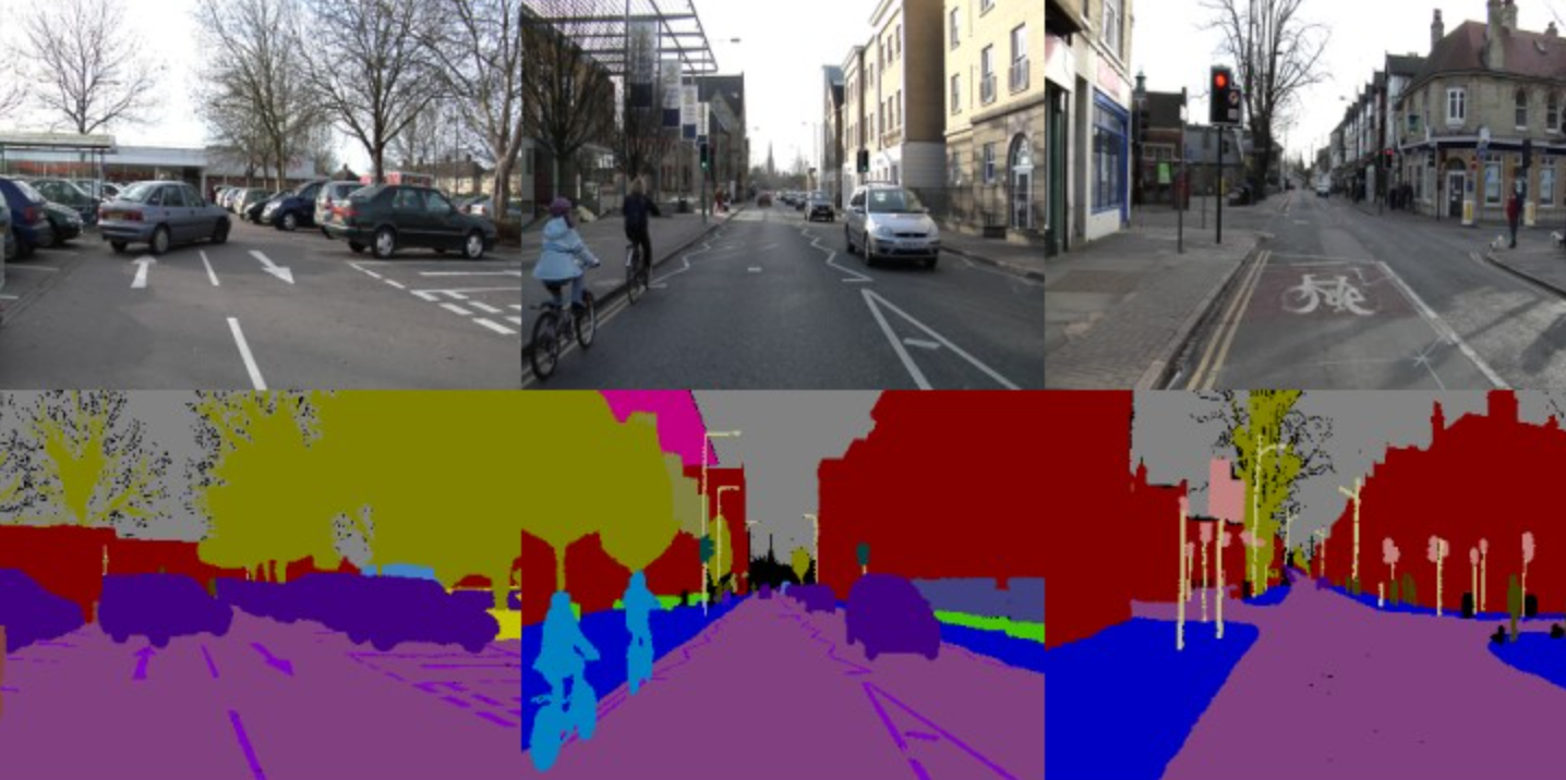 Labeled frames from the CamVid dataset. Each color in the label images corresponds to a
different class.
Labeled frames from the CamVid dataset. Each color in the label images corresponds to a
different class.
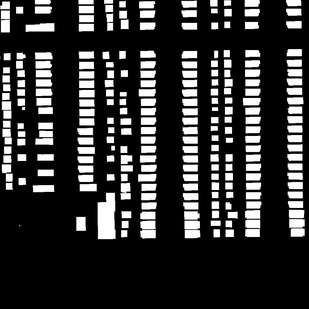
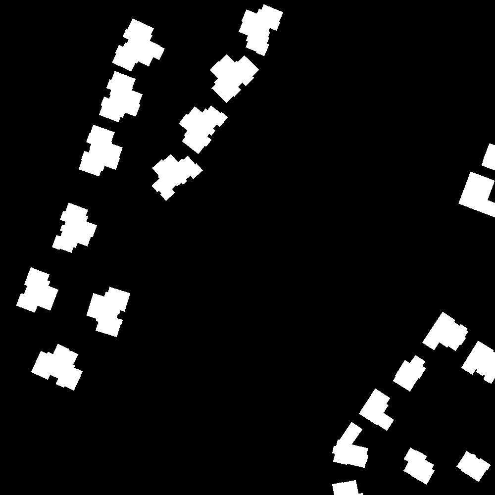
One application of semantic segmentation is the labeling of satellite imagery into classes based on land use. The Inria Aerial Image Labeling Dataset is a collection of aerial images covering several cities from around the world, ranging from densely populated areas to alpine towns, accompanied by ground truth data for two semantic classes: “building” and “not building”. In other words, the Inria dataset can be used to train a pixelwise classifier that can identify human-made structures from satellite images.
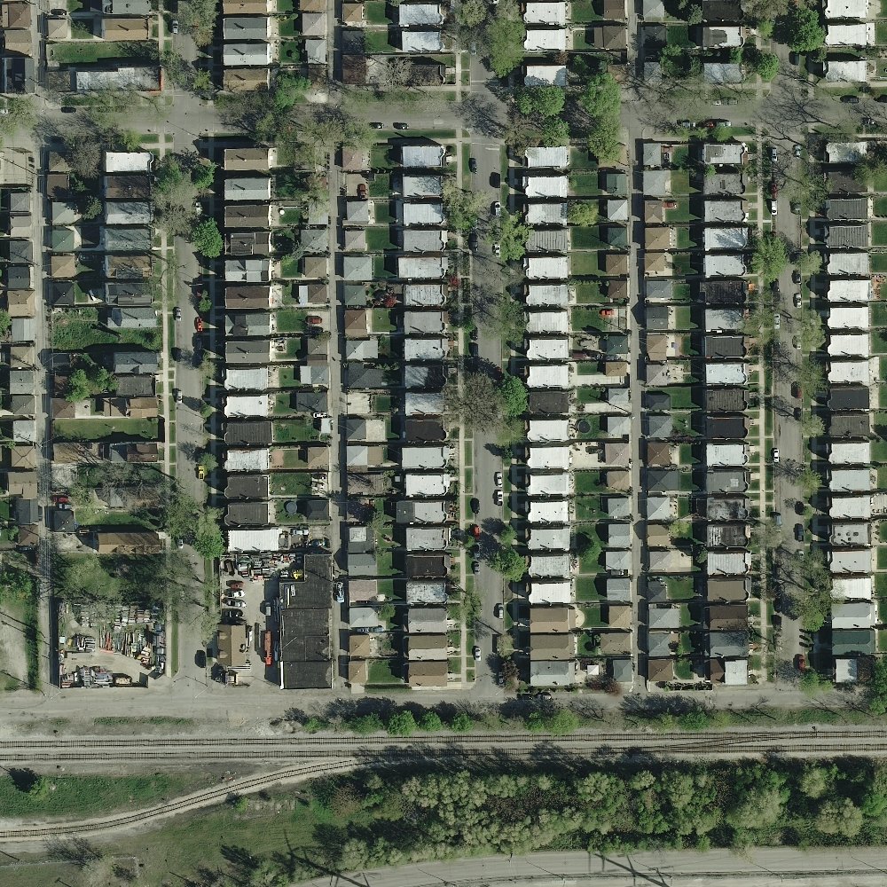
Chicago
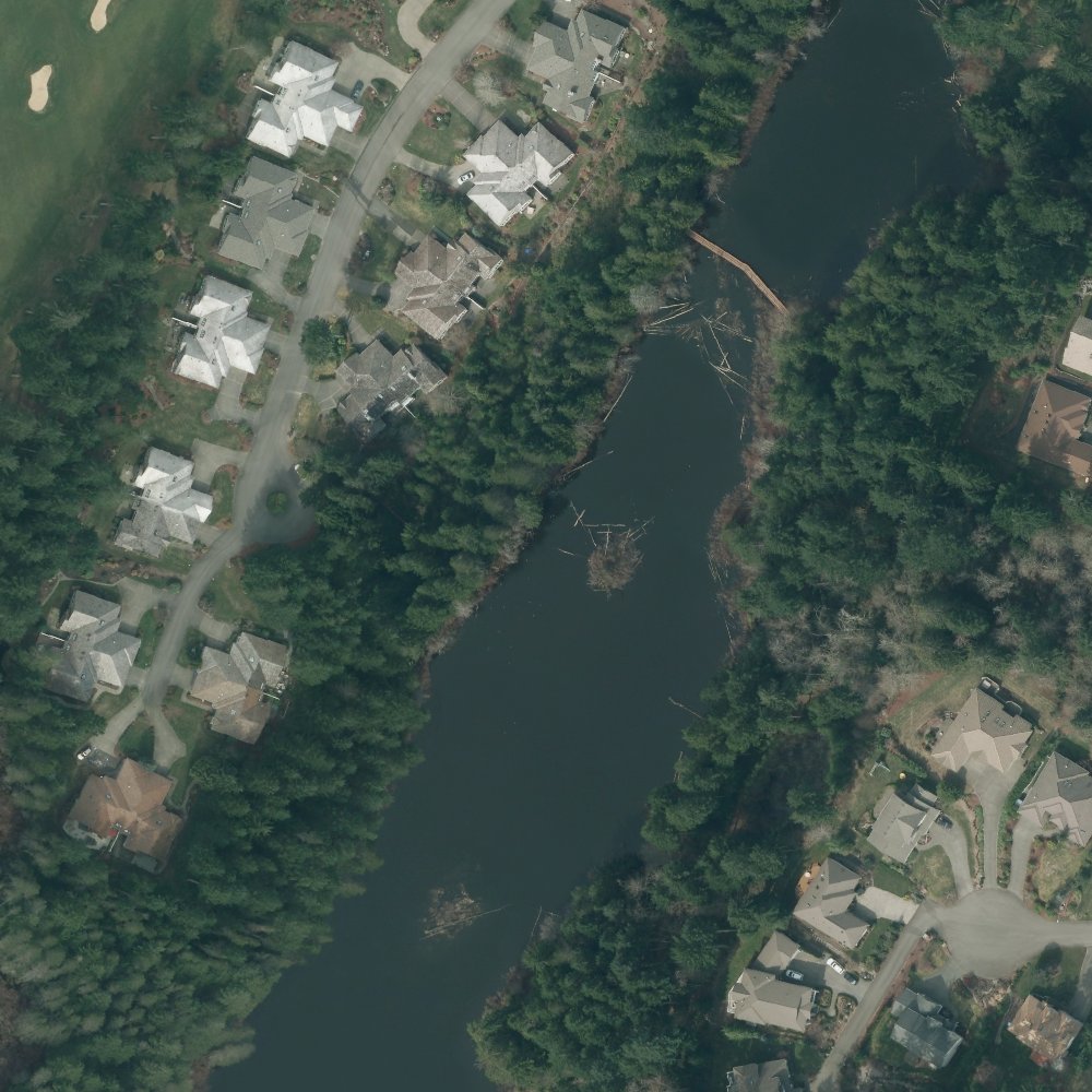
Kitsap County, WA
Images from the Inria dataset with their corresponding labels.
Fast.ai covers semantic segmentation for the CamVid dataset in their Practical Deep Learning for Coders course. After taking the course, I wanted to see if I could apply what I’d learned by using the Fast.ai library and a pretrained ImageNet classifier to train a model on the Inria dataset with competive performance. This post documents my work on the project, including some techniques I learned for working with large format satellite imagery and experimenting with custom model architectures using the Fast.ai library.
The Inria Dataset
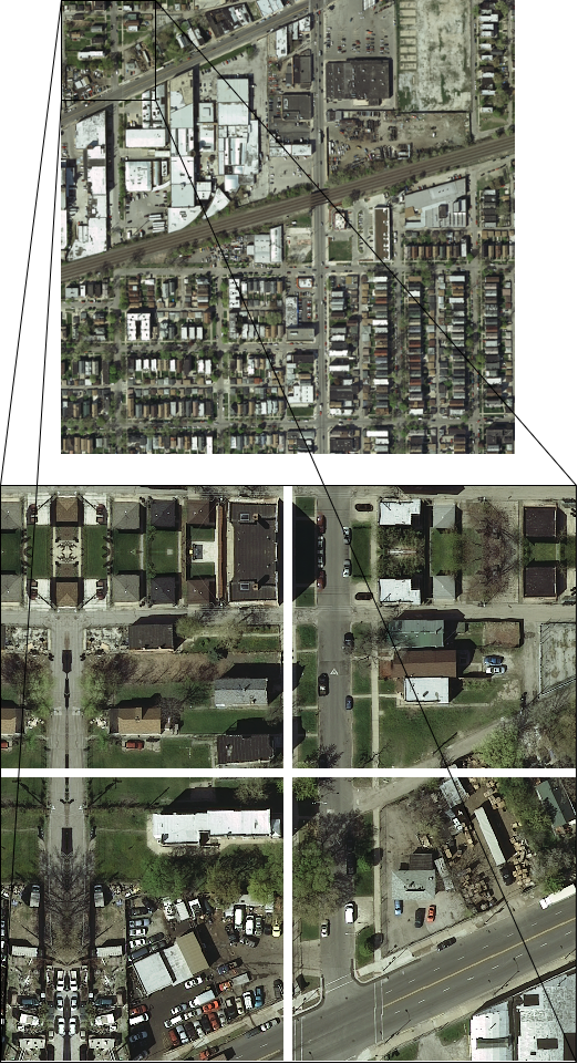
As described above, the Inria dataset is a collection of satellite images covering 10 different cities around the world. Each image, or tile, is a 5000 by 5000 pixel color image that covers an area of 2.25 km2, so the width of a single pixel corresponds to 0.3 m. Half of the images are accompanied by ground truth data, which are single channel images of the same size where pixels corresponding to the building class have value 255 and all others have value 0. These images are used for model training and validation, while the unlabeled images are used as a test set. There is no overlap in cities in the train and test sets; each subset contains 36 images from 5 different cities for a total of 180 images. The authors of the dataset maintain a leaderboard for performance over the test set according to the metrics described below. As suggested by the authors, I used the first tile from each city in the training set for validation.
Given the size of the images relative to available GPU memory, each tile and its label was split up into patches as a preprocessing step. I chose a patch size of 256 by 256 pixels, which allowed me to use a batch size of 32 during training on a single Nvidia Tesla T4 GPU. I used reflection padding to enlarge the tiles so that they could be evenly split into patches. Given the importance of context in identifying building pixels, I used larger, overlapping patches for the validation and test sets, in a process that is described in more detail below.
Patches from one of the tiles in the Inria dataset. Notice the reflection padding in the
edge patches.
Metrics
The evaluation metrics used in the Inria competetion are pixelwise accuracy and intersection over union (IoU) of the building class. IoU is a common evaluation metric in both semantic segmentation and object detection tasks that is defined as the size of the intersection between the predicted and ground truth pixel areas or bounding boxes and the size of their union.
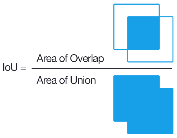 Intersection over Union is defined as the area of overlap between two sets or areas divided by the
area of their union. Image courtesy of
this
blog post by Adrian Rosebrock.
Intersection over Union is defined as the area of overlap between two sets or areas divided by the
area of their union. Image courtesy of
this
blog post by Adrian Rosebrock.
You’ll notice from the competition leaderboard that the accuracy values are generally quite high: all are over 93%. This is partially due to the class imbalance in the dataset. Approximately 15% of the pixels in the training set belong to the building class, so a model that predicted “not building” for all pixels would have an accuracy of around 85%. IoU for the building class, on the other hand, effectively normalizes for the size of the building class to give a measurement of how well the model actually identifies buildings. For that reason, I focused mainly on optimizing IoU over the validation set.
For training I used cross entropy loss, which is the default for semantic segmentation in fastai. I also experimented with soft dice loss, an alternative loss function originally introduced for medical image segmentation which, like IoU, normalizes for the size of each class in the calculation. I expected this to give me a better IoU as it seemed to be more directly optimizing the quantity of interest, but I was not able to beat the performance of a model trained with cross entropy loss. I didn’t look into this in too much detail, but I suspect the dynamics of training with soft dice loss were somehow making it harder for the model to converge to a minimum that would generalize well.
Calculation of soft dice loss. The scoring is repeated over all classes and averaged.
Validation and Test
Given the importance of surrounding context in identifying building pixels, I used a patch size of 1024 by 1024 for the validation and test sets, with 50% overlap between each of the patches. The overlap ensures that each pixel in the test tiles is contained in a patch with at least 25% of the patch size of context in each direction (except for pixels near the tile edges). To produce a prediction map for the tile, the predictions for all of the patches were stitched together and a weighted combination was taken of overlapping pixels, with pixels near the patch edges downweighted.
I took this idea from the leading solution on the Inria leaderboard by Chatterjee and Poullis, but rather than downweighting pixels based on the distance to the nearest edge as they suggest, I went with a slightly different approach. Intuitively it seems like there is some relevant context area around each pixel, and that the weight given to a pixel should be proportional to the ratio of its available context in the patch to the context area. In practice this downweights pixels in the corner of each patch more than those along the center of an edge. In my implementation I chose to specify this context area as a percentage of the overall patch area and found empirically that using a value of 80% (i.e. start to downweight pixels with less than 80% of the entire patch area in context) gave the best performance over the validation set.
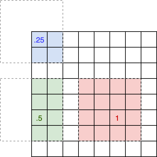
Given a context area, here drawn with a dotted line, centered around each pixel, the pixel weight
is the proportion of that area contained in the patch. The size of the context area is specified as
a proportion of the patch size, in this example it is 50%.
Finally, to assign a predicted class to each pixel we have to apply a threshold to the score output by the model. Here I used Scikit-learn to produce an ROC curve using all pixels in the validation set for a range of thresholds, and derived the accuracy and IoU metrics at those thresholds using the true and false positive rates as well as the counts of positive (building) and negative (not building) samples. I chose the threshold that gave the highest IoU over the validation set.
import sklearn.metrics as skm

def acc_iou_curves(y_true, y_score):
    fpr, tpr, thresholds = skm.roc_curve(y_true, y_score)
    num_pos = (y_true == 1).sum().item()
    num_neg = len(y_true) - num_pos

    fp = fpr * num_neg
    tp = tpr * num_pos
    fn = (1 - tpr) * num_pos
    tn = (1 - fpr) * num_neg

    acc = (tp + tn) / (tp + tn + fp + fn)
    iou = tp / (tp + fp + fn)
    return acc, iou, thresholds
Using an ROC curve to identify the optimal threshold over our validation metrics.
Model Improvements
Fastai includes an implementation of the U-Net architecture for semantic segmentation with a handful of optimizations and smart defaults. After getting to know the dataset better and applying the techniques above to optimize the validation performance, I wanted to see if I could improve on the default U-Net architecture for the Inria dataset. The constraints that I gave myself, in the spirit of the Fast.ai philosophy, were to use a pretrained encoder and avoid distributed training with expensive hardware (I ran all experiments on GCP with a single Nvidia Tesla T4 GPU).
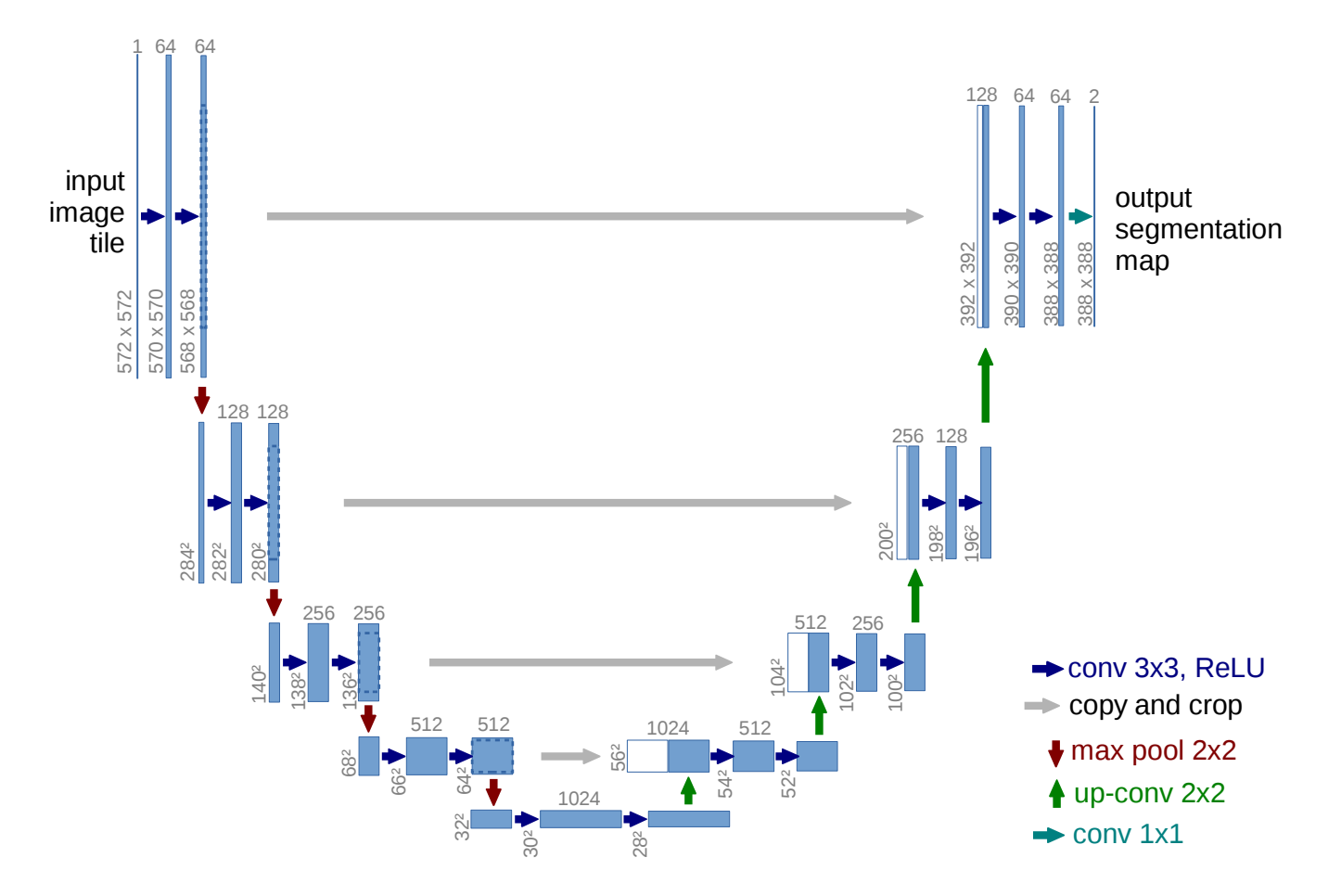 U-Net architecture from the original paper by Ronneberger, Fischer, and Brox. The left side of the
model is the encoder, while the right side is the decoder.
U-Net architecture from the original paper by Ronneberger, Fischer, and Brox. The left side of the
model is the encoder, while the right side is the decoder.
In their leading Inria paper, Chatterjee and Poullis describe a U-Net like model architecture combining a couple ideas from other successful CNN architectures: dense blocks and squeeze and excitation (SE) modules. SE modules were introduced in a 2019 paper by Hu et al. for image classification and allow the network to model the interdependencies between channels of convolutional features using spacially global information from each channel. The modules output a scalar feature for each channel which is used to reweight the feature maps of the block to which they are attached.
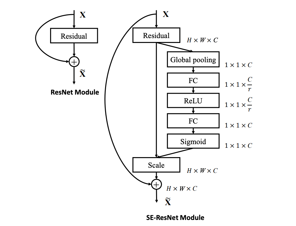 Schema of the squeeze and excitation (SE) module compared to a regular ResNet module, as proposed
by Hu et al.
Schema of the squeeze and excitation (SE) module compared to a regular ResNet module, as proposed
by Hu et al.
Although I was unable to find a pretrained encoder using the exact same architecture described by Chatterjee and Poullis, I did find, in a helpful repo of PyTorch image models, a pretrained SE-ResNet ImageNet classifier, an architecture proposed in the original SE paper, along with an implementation for SE modules. All that remained was to add the SE modules to the decoding path. Doing so with the fastai library required writing a custom model which borrowed heavily from the built-in U-Net implementation but allowed me to attach SE modules to the output of each block. Although this was only a small modification to the network architecture, there were a few details to take care of to ensure compatibility with the fastai library, including: wiring up the cross connections from the encoding to decoding path using PyTorch hooks, ensuring that the “head” or last layer of the pretrained classifier was properly detached to create the encoding path, and ensuring that the layers of the final model were properly grouped to behave reasonably with fastai’s freezing and unfreezing behavior and differential learning rates.
Adding the SE modules gave me a nice performance boost on the validation set, validating the effectiveness that small architectural tweaks can have even without adding a large number of parameters to the model. I also experimented with a DenseNet encoder (without SE modules) and dense block decoder (both with and without SE modules), but found that the SE-ResNet based architecture performed the best. I trained the model frozen (i.e. only updating the decoder weights) for 6 epochs and, after reducing the learning rate, unfrozen for another 10. Each epoch took approximately 50 minutes to train on the Tesla T4. I submitted my test set results to the competition and scored an overall IoU of 74.84, which put me in the top 25% of the leaderboard. Not bad for less than 14 hours of training!
Conclusion
Building a semantic segmentation model for satellite imagery was challenging primarily due to the size of the input images. After learning how to break the images up and reassemble the model output, however, I found that the fastai library makes it easy to get up and running with close to state of the art performance on semantic segmentation tasks, by encouraging the use of pretrained ImageNet models and providing an opinionated workflow for model development. Modifying the library’s defaults was a little challenging at times (for example using a different image size for the validation and test sets and needing to rewrite most of the U-Net implementation), but, especially as somebody relatively new to deep learning, it was useful to have a baseline that I knew was going to give me good performance and to be able to iterate from there. This project gave me the opportunity and motivation to discover as necessary the details required to improve performance on this particular problem, and I would highly recommend using personal projects to deepen your own understanding of the Fast.ai material.
All of the code for this project can be found in a notebook on my GitHub.
References
[1] Brostow, Fauqueur, Cipolla. “Semantic Object Classes in Video: A High-Definition Ground Truth Database”. Pattern Recognition Letters.
[2] Emmanuel Maggiori, Yuliya Tarabalka, Guillaume Charpiat and Pierre Alliez. “Can Semantic Labeling Methods Generalize to Any City? The Inria Aerial Image Labeling Benchmark”. IEEE International Geoscience and Remote Sensing Symposium (IGARSS). 2017.
[3] Practical Deep Learning for Coders.
[4] Milletari, Navab, Ahmadi. “V-Net: Fully Convolutional Neural Networks for Volumetric Medical Image Segmentation”. 3DV 2016.
[5] Chatterjee, Poullis. “Semantic Segmentation from Remote Sensor Data and the Exploitation of Latent Learning for Classification of Auxiliary Tasks”.
[6] Ronneberger, Fischer, Brox. “U-Net: Convolutional Networks for Biomedical Image Segmentation”. MICCAI 2015.
[7] Hu, Shen, Albanie, Sun, Wu. “Squeeze-and-Excitation Networks”. CVPR 2018.